
How many Bluetooth beacons I can have in one place?
Every now and then someone asks how many RuuviTag Bluetooth sensor beacons they can have in range of a single gateway. Is it feasible to monitor every box in a warehouse? Every individual carton of milk inside those boxes?
It turns out that there is no exact answer, as the data is sent in stand-alone packets. The question becomes: What is the rate at which Bluetooth Low-Energy (BLE) packets can be received?
Theoretical maximum of Bluetooth beacons
Bluetooth advertisements are on three separate frequency channels, known as 37, 38 and 39. Texas Instruments has an excellent primer about the channels and advertising in case you’re interested in deeper details.
Minimum advertisement packet size is 80 bits (or 10 bytes), containing:
- Preamble: 1 byte
- Access address: 4 bytes
- Header: 2 bytes
- CRC: 3 bytes
Assuming we want to just fill the spectrum with valid BLE advertisement data, and somehow we get every device in perfect synchronization we could be broadcasting these packets on every channel and receive each channel separately. The limiting factor would be the data rate of BLE 4, which is
1 Mbit / s.
Total would be 1 000 000 bit / s divided by 80 bit / s times 3 channels, or
37 500 transmissions per second. However, there are numerous practical limits, starting with our gateway which probably scans on only one channel.
Practical limits to packet rate in Bluetooth
Channels
As the sensor beacons are delivered as a single component, rather than an integrated system, we need to advertise on all of the channels to be sure to hit whichever channel our gateway happens to be listening to. As we must send the same advertisement on every channel, we cannot use multiplexing over three channels and the 37 500 transmissions are divided by three down to 12 500.
Data size
Our initial assumption was that data size of a packet is 80 bits. However, that’s not useful at all — those 80 bits don’t even include the MAC address of the beacon. Let us be more careful with data size estimate, and use full 376 bits of BLE 4 advertisement. This limits us to 2 659 packets per second.
Synchronization
Bluetooth does not come with a mechanism to synchronize the beacons to divide the bandwidth equally among all devices. The beacons instead advertise at random moment, hoping to miss any other disturbance at least most of the time. Naturally chance of missing any other packet decreases as the traffic in the bands increase. Nordic Devzone has an excellent answer on estimating the collision probability: Essentially we assume that if any two packets collide on a channel, both are lost. Collision probability is calculated between two advertisers based on air time of a packet and the interval between transmitting.
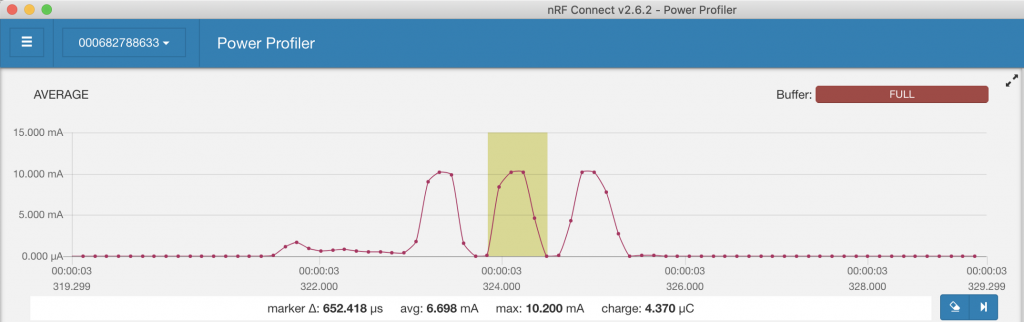
While the theoretical model based on modulation speed predicts that a single broadcast on a single channel takes 376 microseconds, we’ll get a bit more practical and measure the time from the current ramp-up to the ramp-down in an advertisement. The results are somewhat varied as they depend on the exact moment sample is taken, but we’ll pick 650 microseconds as our measured value.
We’ll select one second as our interval as we’re trying to figure out how many advertisements we can receive in a second. Our probability to collide packets P(hit) becomes 2 * 65e-5 / 1, which equals to 0.13 %. Our probability to not hit other packet P(miss) is then 1- P(hit), or 99,87 %.
As the beacons are independent, we can calculate the probability of not hitting any of N beacons as a compound probability of not hitting one beacon: P(miss_all) = P(miss)^N-1. We’ll plot the total throughput of beacons sending packets once per second with Scilab.
N = 1:1:5000;
throughput = zeros(1, 5000);
Pmiss = 1 - (2*65*10^-5);
for i=1:1:length(N)
  Pmiss_all = Pmiss^(i-1);
  throughput(1, i) = i * Pmiss_all;
end
plot(N, throughput)
[v, i] = max(throughput)
a = gca();
a.font_size = 5;
a.x_label.text = string("Number of beacons") ;
a.x_label.font_size = 6;
a.y_label.text = "Throughput (N/s)";
a.y_label.font_size = 6;
e=gce();
p1=e.children(1);
t=datatipCreate(p1,769);
t.font_size = 5;
Gateway and background noise
In addition to beacons themselves, there is always some background noise which limits the number of packets we can receive. Likewise the gateway itself might use shared antenna for WiFI and Bluetooth. In practice I’ve seen gateways to have 5 % to 50 % packet loss in otherwise good conditions. Assuming the gateway can listen to 100 % of advertisements and background is otherwise quiet, we might receive 95 % of non-colliding packets or 268 transmissions per second — quite a difference to the theoretical maximum of 37 500!
Backend and connectivity
While the Bluetooth payload data rate is not extreme by any means — only some 12 kB/s in the above case — actual internet traffic might be a whole lot more, especially if data is written with separate connections for each data point rather than by dumping a few thousand points at a time. However, performance of different backend solutions is outside the scope of this post.
So, how many Bluetooth beacons I can deploy after all?
There is no simple answer, so we’ll have to say “it depends”. The above graph suggests that even with 5000 beacons sending data once per second some data would get through, but a chance of a transmission being received is only 0.15 %. On average one out of 668 transmissions would be received — that’s 11 minutes. The limiting factor becomes how long I can wait to receive a transmission with high enough certainty.
Let’s say that we’re monitoring temperature and humidity inside a warehouse. Waiting 11 minutes might be entirely safe, as neither of those values change rapidly under common conditions. On the other hand, if the beacons are used for inventory tracking inside a warehouse, we might have only 10 seconds near gateway before the goods are driven off.
We’ll pick 2 thresholds for the certainty of detecting a tag within given time: a strict 99.99999 % for mobile inventory tracking and a lot more relaxed 99 % for tracking conditions of a static asset. Let’s fix the other variables as well.
- Transmission time: 650 microseconds
- Interval: 1 second
- Gateway, background noise: 5 % of packets are lost
Next we calculate a matrix of detection probabilities within given time, find the first time which has greater probability than our threshold and plot the times on Scilab.
Ttransmission = 65e-5;
Tinterval = 1;
Penvironment = 0.95;
Ntags = 1:1:5000;
Pmiss = 1 - (2*Ttransmission/Tinterval);
Pmiss_all = Pmiss^(Ntags - 1) * Penvironment;
Pnot_miss_all = 1-Pmiss_all;
Nbroadcasts = 1000;
for i=1:1:Nbroadcasts
  Pnot_detect(i, :) = Pnot_miss_all^i;
end
Pdetect = 1 - Pnot_detect;

th1 = 0.99;
th2 = 0.9999999;
[idx, idy] = find(Pdetect > th1);
[uniq, map] = unique(idy);
plot(1:1:length(map), idx(map));
[idx2, idy2] = find(Pdetect > th2);
[uniq2, map2] = unique(idy2);
plot(1:1:length(map2), idx2(map2), 'g');

a = gca();
a.font_size = 5;
a.x_label.text = string("Number of beacons") ;
a.x_label.font_size = 6;
a.y_label.text = "Time to detect with probablity (s)";
a.y_label.font_size = 6;

hl = legend(["99 %", "99.99999 %"], 2);
hl.font_size = 5;
Now we can pick some examples for beacon densities. On a warehouse scenario, where we want to detect the beacon data once per minute with 99 % certainty, we can have some 1900 beacons broadcasting once per second.
In inventory tracking scenario, where we want to detect the transmission in 10 seconds with 99.99999 % certainty, we can have 100 beacons in range.
Verifying the estimates
Any good theory can be tested for correctness. Verifying these examples shouldn’t be too hard, all we need is a Raspberry Pi and a few thousand RuuviTags.

Luckily we can adjust the numbers a bit to verify the base idea so we won’t have to purchase thousands of tags. We’ll speed everything up and use 100 ms interval and check if we get at least one transmission per second from the tags.
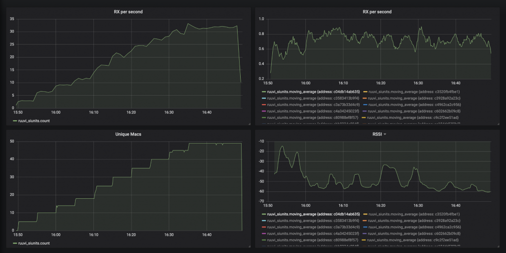
We’ll program 16 beacons to transmit at 100 ms interval and put them next to Raspberry Pi and ESP32 dongle which relay the data to InfluxDB. Raspberry Pi is connected via Ethernet and ESP32 via WiFi.
The end result is quite disappointing: The backend connection gets saturated at some 150 samples per second peak, and no more data can be received.
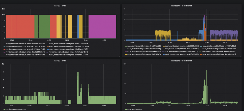
Our next try has a local database running on a PC which should eliminate the backend bottleneck. However, here we run into a bottleneck in scanning: Even when there’s only one tag on we get less than 10 % of advertisements. A quick search on the internet shows that this might be related to Mac OSX BLE scanning firmware and hardware which shares the antenna with WiFi and doesn’t scan 100 % of the time.
Visually it seems that the total throughput was 0.75 with one tag, 4,5 with 8 tags and 11 with 16 tags. The throughput of a single tag was rather constant 0.75 the whole time.
Refining the model
A good thing about our theoretical model is that it does recognize gateway imperfections. We’ll update our estimates with 92 % gateway loss and estimate the reception rate with 51 tags. For a good measure we’ll also use the actual average transmission interval of 105 ms which includes average random delay in our prediction.
A first run shows that the model has faster collision increase rate than we see with transmission time of 650 microseconds, and therefore we set the transmission time to 450 microseconds which is a bit over the theoretical time derived from modulation speed. Now our model matches the experiment pretty well, at least in range of 1 to 16 beacons. We’ll omit the first run results for the sake of brevity.
N = 1:1:60;
throughput = zeros(1, length(N));
Tinterval = 0.105
Ttx = 65*10^-5
Pmiss = 1-(2*Ttx/Tinterval);
Penvironment = 0.080;
for i=1:1:length(N)
  Pmiss_all = Pmiss^(i-1);
  throughput(1, i) = i * Pmiss_all * Penvironment / Tinterval;
end
plot(N, throughput)
[v, i] = max(throughput)
a = gca();
a.font_size = 5;
a.x_label.text = string("Number of beacons") ;
a.x_label.font_size = 6;
a.y_label.text = "Throughput (N/s)";
a.y_label.font_size = 6;
e=gce();
p1=e.children(1);
t=datatipCreate(p1,1);
t.font_size = 5;
t=datatipCreate(p1,8);
t.font_size = 5;
t=datatipCreate(p1,16);
t.font_size = 5;
Now we have a refined model which matches reasonably well to measured real-world data. It’s time to see how the model holds up when we add 51 tags in total.
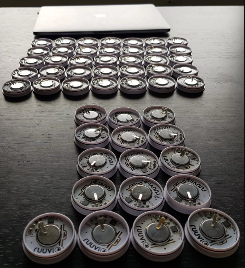
The tags used here are factory rejects, fair showcase samples etc. No Ruuvis were harmed in this experiment. As some of the tags we used for testing couldn’t pass our production testing, two of the tags didn’t broadcast anything at all. Final total of broadcasters was 49.
N = 1:1:60;
throughput = zeros(1, length(N));
throughput_single = zeros(1, length(N));
throughput_measured = [ 3, 6.5, 9.1, 11.2, 16.9, 20, 24.6, 27.2, 29.5, 31.9 ];
throughput_samples = [ 5, 10, 14, 18, 25, 30, 35, 40, 45, 49 ];
Tinterval = 0.105
Ttx = 45*10^-5
Pmiss = 1-(2*Ttx/Tinterval);
Penvironment = 0.080;
for i=1:1:length(N)
  Pmiss_all = Pmiss^(i-1);
  throughput(1, i) = i * Pmiss_all * Penvironment / Tinterval;
  throughput_single(1, i) = Pmiss_all * Penvironment / Tinterval;
end
plot(N, throughput)
plot(throughput_samples, throughput_measured, 'g')
a = gca();
a.font_size = 5;
a.x_label.text = string("Number of beacons") ;
a.x_label.font_size = 6;
a.y_label.text = "Throughput (N/s)";
a.y_label.font_size = 6;
hl = legend(["Estimated", "Measured"], 2);
hl.font_size = 5;
Curiously there isn’t a noticeable effect of less packets being received when we add more beacons. Maybe the firmware in my Macbook rate limits results if they come in at extreme rate, and we keep receiving packets at the maximum rate supported by my hardware?
We can take another approach to determine the reliability. We leave 46 beacons on overnight, and check the number of 10 second intervals where at least one beacon was not seen.
Over the course of 10 hours there is 3600 10-second intervals, and we have 46 beacons for a total of 165 600 samples of a beacon transmitting data for 10 seconds. On 70 of these samples, no data was received.
A reliability calculator gives us 99.99% confidence of 99.94 % reliability of receiving data within 10 second interval. We’ll cross-check this result with our earlier reliability estimator.
Ttransmission = 65e-5;
Tinterval = 0.1;
Penvironment = 0.95;
Ntags = 1:1:50;
Pmiss = 1 - (2*Ttransmission/Tinterval);
Pmiss_all = Pmiss^(Ntags - 1) * Penvironment;
Pnot_miss_all = 1-Pmiss_all;
Nbroadcasts = 1000;
for i=1:1:Nbroadcasts
  Pnot_detect(i, :) = Pnot_miss_all^i;
end
Pdetect = 1 - Pnot_detect;

th1 = 0.9994;
[idx, idy] = find(Pdetect > th1);
[uniq, map] = unique(idy);
plot(1:1:length(map), idx(map));

a = gca();
a.font_size = 5;
a.x_label.text = string("Number of beacons") ;
a.x_label.font_size = 6;
a.y_label.text = "Time to detect with probablity (s)";
a.y_label.font_size = 6;

hl = legend(["99.94 %"], 2);
hl.font_size = 5;
Curiously our reliability estimator is spot-on with the measurements, while the packet loss rate was wildly off. One possible cause is that Macbook BLE firmware collects several transmissions from same MAC into a batch and reports only rate-limited results to higher levels of OS and applications.
Conclusions
The original question was: How many beacons I can have in one area? For most of the people, we can confidently say Enough. We had up to 46 beacons transmitting at 100 ms interval and we could hear them all at relatively fast rate and good reliability.
If the results can be scaled to slower intervals and larger number of beacons, we could estimate that 460 beacons transmitting at 1 s interval could be heard within 100 seconds and 4600 beacons transmitting at 10s interval could be heard within 1000 seconds with pretty good reliability. However this estimate is not backed up by an experiment.
Models for packet loss could not be verified because most of the packets were not received by our receiving hardware for yet unknown reason. A follow-up with dedicated scanning hardware and software has to be made to verify those estimates.
Stay tuned for a follow-up post with dedicated nRF52 scanners and multiple MAC address broadcasting tags which will let us get more precise results on the limits of broadcasters in the area.
Thanks to Lauri Jämsä.